Onsager’s solution of the 2-D Ising model: The combinatorial method

1. Introduction

In this blog post, I derive, step by step, the exact partition function for the ferromagnetic Ising model on the square lattice. The result is celebrated as “Onsager’s solution” of the 2-D Ising model. It was originally derived by Lars Onsager in 1942 and published in 1944 in Physical Review [1]. That paper revolutionized the study of phase transitions and what we now call critical phenomena [2].

Somewhat ironically, I first heard about the Ising model when I was working in industry. I was 20 and held a summer job at what was then known as British Telecom Research Labs (BTRL), near Ipswich in the UK. This was before I had ever seen a cell phone or heard of the Internet (although I knew about BITNET and JANET). I worked there in the summer of 1990 and again for a month or so around April 1991. My job at BT involved writing C implementations of multilayer perceptrons and Hopfield neural nets. In those days, BT was interested in implementing hardware neural networks and my boss mentioned casually to me that certain kinds of neural nets are basically just special cases of the Ising model. (Indeed, the Hopfield network is closely related to the Ising spin glass.) Thus began my fascination with the Ising model. Later, in 1994 in Boston, I took a course given by Bill Klein at BU on statistical mechanics, where we went through the solution of the 1-D ferromagnetic Ising model. Still, I never had the chance to study properly the 2-D Ising model. As a PhD student, I would almost daily pass by a poster with a background photo of Lars Onsager (with a cigarette in his hand), hung near the office door of my advisor Gene Stanley, so I was regularly reminded of the 2-D Ising model. I kept telling myself that one day I would eventually learn how Onsager managed to do what seemed to me, at the time, an “impossible calculation.” That was 1994 and I am writing this in 2015!

In what follows, I solve the Ising model on the infinite square lattice, but I do not actually follow Onsager’s original argument. There are in fact several different ways of arriving at Onsager’s expression [3–9]. The method I use below is known as the combinatorial method and was developed by van der Waerden, Kac and Ward among others and relies essentially on counting certain kinds of closed graphs (see refs. [3,10–13]). I more or less follow Feynman [3] and I have also relied on the initial portions of ref. [13].

2. The 2-D Ising model

Consider a two dimensional lattice ${\Bbb Z^2}$ where at each point of the lattice is located a (somewhat idealized) spin- ${\tfrac{1}{2}}$ particle. Consider a finite subset of this lattice, of size ${L\times L}$ and let ${i,j=1,2,\ldots L^2}$ . Let ${\cal N}$ denote the set of pairs of integers ${(i,j)}$ such that spins ${\sigma_i}$ and ${\sigma_j}$ are nearest neighbors. In the ferromagnetic 2-D Ising model with nearest neighbor interactions, spins ${i}$ and ${j}$ interact if and only if ${(i,j)\in \cal N}$ . Each spin ${\sigma_i}$ can assume only 2 values: ${\sigma=\pm 1}$ .

Consider a system of ${N=L^2}$ spins. The Hamiltonian for a spin configuration ${\sigma=(\sigma_1,\sigma_2,\ldots \sigma_N)}$ is given by

$\displaystyle H(\sigma)= -J \displaystyle\sum_{i,j\in \cal N} \sigma_i \sigma_j ~. \ \ \ \ \ (1)$

The sum over the nearest neighbors should avoid double counting, so that ${(i,j)}$ and ${(j,i)}$ are not counted separately. Without loss of generality, we will assume ${J=1}$ for simplicity.

3. The canonical partition function

In the theory of equilibrium statistical mechanics, the canonical partition function contains all the information needed to recover the thermodynamic properties of a system with fixed number of particles, immersed in a heat bath, details of which can be found in any textbook on statistical mechanics [3-6,14].

I prefer to define the partition function as the two-sided Laplace transform of the degeneracy ${\Omega(E)}$ of the energy level ${E}$ . But traditionally, the partition function is defined as a sum or integral over all possible states of the system:

$\displaystyle Z(\beta) = \displaystyle\sum _{\sigma} e^{-\beta H(\sigma)} ~. \ \ \ \ \ (2)$

The two ways of thinking are equivalent. The Laplace transform variable ${\beta}$ is related to the thermodynamic temperature ${T}$ via ${\beta =1/k_B T}$ , where ${k_B}$ is the Boltzmann constant. What follows is the exact calculation of ${Z(\beta)}$ .

4. The partition function of the 2-D Ising model

The sum over the full configuration space spans over exactly ${2^N}$ states, because each spin can only have 2 possible values. Moreover, since the sum is finite (for finite ${N}$ ), we can write the ${N}$ -sum as ${N}$ iterated sums, to obtain

$\displaystyle Z= \displaystyle\sum_{\sigma_1=\pm 1} \displaystyle\sum_{\sigma_2=\pm 1} \ldots \displaystyle\sum_{\sigma_N=\pm 1} e^{-\beta H(\sigma)} ~.\ \ \ \ \ (3)$

Let us rewrite the exponential factor as

$\displaystyle e^{-\beta H}= \exp[\beta \displaystyle\sum_{\cal N} \sigma_i \sigma_j]=\displaystyle\prod_{\cal N} \exp [\beta \sigma_i\sigma_j] ~. \ \ \ \ \ (4)$

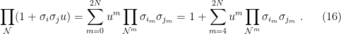
So we get for the partition function

$\displaystyle Z= \displaystyle\sum_{\sigma_1=\pm 1} \displaystyle\sum_{\sigma_2=\pm 1} \ldots \displaystyle\sum_{\sigma_N=\pm 1} \displaystyle\prod_{\cal N} \exp [\beta \sigma_i\sigma_j] ~. \ \ \ \ \ (5)$

Next, consider that ${\sigma_i\sigma_j}$ can only assume the two values ${\pm 1}$ . Moreover, ${e^{\pm \beta}= \cosh(\beta) \pm \sinh(\beta)}$ , so that

$\displaystyle \displaystyle\prod_{\cal N} \exp [\beta \sigma_i\sigma_j] = \displaystyle\prod_{\cal N} (\cosh (\beta) + \sigma_i \sigma_j \sinh (\beta)) ~. \ \ \ \ \ (6)$

We will next carry out a change of variables to eliminate the hyperbolic functions. Let us write

$\displaystyle \cosh (\beta) + \sigma_i \sigma_j \sinh (\beta)= \cosh (\beta)(1 + \sigma_i \sigma_j \tanh (\beta))= \cosh (\beta)(1 + \sigma_i \sigma_j u) \ \ \ \ \ (7)$

where ${u=\tanh(\beta)}$ . From the identity

$\displaystyle 1-\tanh^2(x)={\rm sech}^2(x) \ \ \ \ \ (8)$

we get

$\displaystyle \displaystyle { 1 \over \sqrt{1-u^2}}= \cosh(\beta) \ \ \ \ \ (9)$

so that

$\displaystyle \begin{array}{rcl} \displaystyle\prod_{\cal N} (\cosh (\beta) + \sigma_i \sigma_j \sinh (\beta)) &=& \displaystyle\prod_{\cal N} (1+\sigma_i \sigma_j u) /\sqrt{1-u^2} \\ &=& (1-u^2)^{-n_b/2} \displaystyle\prod_{\cal N} (1+\sigma_i \sigma_j u) \end{array}$

where ${n_b=|{\cal N}|=2N}$ is the number of total bonds, assuming periodic boundary conditions. So we finally get

$\displaystyle Z= (1-u^2)^{-N} \displaystyle\sum_{\sigma_1=\pm 1} \displaystyle\sum_{\sigma_2=\pm 1} \ldots \displaystyle\sum_{\sigma_N=\pm 1} \displaystyle\prod_{\cal N} (1+\sigma_i \sigma_j u) ~. \ \ \ \ \ (10)$

To proceed further, we must now evaluate the product that appears inside the summation. Expanding the product, we can write

$\displaystyle \displaystyle\prod_{\cal N} (1+\sigma_i \sigma_j u) = (1+\sigma_{i_1} \sigma_{j_1} u) (1+\sigma_{i_2} \sigma_{j_2} u) \ldots \ \ \ \ \ (11)$

as a polynomial in ${u}$ . Collecting the monomial terms ${u^m}$ , we can write

$\displaystyle \displaystyle\prod_{\cal N} (1+\sigma_i \sigma_j u) =\displaystyle\sum_{m=0}^{2N} u^m \displaystyle\prod_{{\cal N}^m} \sigma_{i_m} \sigma_{j_m} ~. \ \ \ \ \ (12)$

The summation is over ${m}$ distinct nearest neighbor pairs, of which there are exactly ${2N}$ , i.e. the number of bonds.

Recall that a graph is a collection of nodes or vertices connected by edges or links. Given any collection of bonds, we can treat the bonds as edges and the spins connected to those bonds as the nodes. So in the language of graph theory, we can say that the last summation above is over all graphs with ${m}$ edges, i.e. ${m}$ bonds. The maximum valence or degree of a node in the 2-D Ising model is 4.

Now, observe that if a node ${\sigma_k}$ has degree ${q_k}$ in some particular graph of ${m}$ bonds, then ${\sigma_k}$ appears ${q_k}$ times in the product over the graphs of ${m}$ bonds. Consider nodes with odd degree ${q_k}$ . In the iterated summation over all spin configurations, there is one sum over ${\sigma_k=\pm 1}$ . Since

$\displaystyle \displaystyle\sum _{\sigma_k=\pm 1} \sigma^{q_k}= -1+1=0 ~, \ \ \ \ \ (13)$

therefore any graph with even a single node of odd degree will have a zero factor, eliminating its contribution to the partition function. So the sum over graphs of ${m}$ bonds need include only graphs with nodes of degree 2 and 4. Indeed, for even degree ${q_k=2,4}$

$\displaystyle \displaystyle\sum _{\sigma_k=\pm 1} \sigma^{q_k}= 1+1=2 ~. \ \ \ \ \ (14)$

So for the graphs of nodes of even degree, each node contributes a factor 2. If the graph of ${m}$ bonds has ${V}$ vertices or nodes, then that graph will contribute a factor ${2^V}$ . There are also ${N-V}$ spins which are not counted in the graph of ${m}$ bonds. The summation over these leftover spins can be summed separately. For each such spin ${\sigma_i}$ we get

$\displaystyle \displaystyle\sum_{\sigma_i=\pm 1} 1 =2 \ \ \ \ \ (15)$

so that we get an additional factor ${2^{N-V}}$ . We get a total factor of ${2^{V+N-V}=2^N}$ . Finally, let us separate the ${m=0}$ case and write

$\displaystyle \displaystyle\prod_{\cal N} (1+\sigma_i \sigma_j u) =\displaystyle\sum_{m=0}^{2N} u^m \displaystyle\prod_{{\cal N}^m} \sigma_{i_m} \sigma_{j_m} =1 + \displaystyle\sum_{m=4}^{2N} u^m \displaystyle\prod_{{\cal N}^m} \sigma_{i_m} \sigma_{j_m} ~. \ \ \ \ \ (16)$

Let us at this point introduce new terminology to refer to graphs only with nodes with even degree and call such graphs admissible graphs. Let us denote the set of all admissible graphs by ${\cal A}$ . We can thus rewrite the partition function as

$\displaystyle Z=2^N (1-u^2)^{-N} \left(1 + \displaystyle\sum_{G\in \cal A} u^{m(G)} \right) ~, \ \ \ \ \ (17)$

where ${m(G)}$ is the number of bonds in admissible graph ${G}$ .

Note that in ${d}$ dimensions, the only difference is that ${n_b=dN}$ so that

$\displaystyle Z_d=2^N (1-u^2)^{-dN/2} \left(1 + \displaystyle\sum_{G\in \cal A} u^{m(G)} \right) ~. \ \ \ \ \ (18)$

In ${d=1}$ dimensions, there are no admissible graphs (if we neglect the boundary conditions) and we immediately recover

$\displaystyle Z_1=2^N \cosh^N(\beta) ~, \ \ \ \ \ (19)$

so that the partition function per spin (see definition further below) is

$\displaystyle \lambda_1=2 \cosh(\beta) ~.\ \ \ \ \ (20)$

5. Summation over paths

We now have the partition function as a sum over admissible graphs. These admissible graphs contain only nodes with even degree, so that dangling nodes are impossible, i.e. the graphs contain only (disconnected or connected) loops. So it makes sense to try to decompose the graphs in terms of closed loops.

Let us consider the bonds between nearest neighbor sites ${i,j}$ as starting at ${i}$ and ending at ${j}$ . In other words, we are orienting the bonds. Let us define a path as a sequence of bonds, such that each bond starts where the previous bond finished, but never going backwards over the previous bond. Moreover, the last bond ends where the first bond started, so that paths are closed by definition.

Since all paths are closed, there are many possible starting (or ending) points, and we are only interested in the equivalence class of paths equivalent up to circular permutation of the bond order. The inverse of a path is defined as the bonds in inverse order and with opposite orientation, in agreement with the usual common sense. We will not distinguish between paths and their inverses, i.e. they are equivalent in what follows.

But now, we are going to assign to every path a positive or negative signature ${\pm 1}$ . Let ${t}$ be the number of windings or rotations made by the tangent vector of a path as it traverses the whole path, i.e. the total angle of rotation divided by ${2 \pi}$ . Angle is measured in the standard convention of counterclockwise being positive. We then define the sign ${s}$ of a path ${p}$ by

$\displaystyle s(p) = - (-1)^t \ \ \ \ \ (21)$

so that if a path goes around an odd number of times, then the sign is positive but if the path winds around an odd number of times, then the sign is negative.

If a path is periodic, we define the period ${w}$ to be the largest integer such that the ${w}$ identical sub-paths are not periodic. If a path is periodic with period ${w}$ , then the sign of the periodic path is defined as

$\displaystyle s(p) = - (-1)^{wt_s} \ \ \ \ \ (22)$

where ${t_s}$ is the value of ${t}$ for the non-periodic subpath. In particular, the sign of a periodic path is not the product of the signs of the subpaths. Instead, the sign of a periodic path is -1 if the period is even. If the period is odd, then the sign of the periodic path equals the sign of the non-periodic subpath.

We now define the “amplitude” or weight of a path ${p}$ as

$\displaystyle W(p)= s(p)u^{m(p)} \ \ \ \ \ (23)$

so that the amplitude can be positive or negative, but its absolute value is ${u^m}$ , where ${m}$ is the total length of the path. Recall that ${u\leq 1}$ for non-negative ${\beta}$ .

Next, consider the infinite product over all equivalence classes ${[p]}$ of closed non-periodic paths

$\displaystyle \displaystyle\prod_{[p]} (1+W(p)) ~. \ \ \ \ \ (24)$

The expansion of the product will contain terms like

$\displaystyle W(p_1)W(p_2)\ldots W(p_k)= s_1 u^{m_1} s_2 u^{m_2} \dots s_k u^{k_k} ~. \ \ \ \ \ (25)$

Let ${s=s_1 s_2 \dots s_k}$ . Let us now decompose the product of all the powers of ${u}$ in terms of how many times the bonds appear in the paths.

Some of the bonds will appear multiple times, because they might be part of two or more distinct paths. Let us consider first the situation where each bond appears at most once in the ${k}$ different paths. This means that either the ${k}$ paths are disjoint, i.e. do not intersect, or else they intersect in a such a manner that no bond is traversed by both intersecting paths. This can only happen if the intersection nodes have degree 4. When a path enters through a bond to a node of degree 4, there are 3 possible exit bonds.

Let ${V_4}$ be the number of nodes with degree 4. Since at each node of degree 4 there are 3 types of path crossings, there are ${3^{V_4}}$ possible choices of path combinations for any given graph. Each such choice of paths will have a sign. Let us take a closer look at all these signed terms.

The 3 types of crossings are (1) straight through, (2) turn clockwise and (3) counterclockwise. Let ${t_i}$ be the number of intersections of type ${i=1,2,3}$ , including self-crossings plus crossings of the ${k}$ different paths. Crossings of type 1 of distinct paths can happen only an even number of times and ${\pm 1}$ to an even power is 1.

Each self-crossing of type 1 means that 1 full rotation of the tangent vector has been made. So we get a sign contribution ${(-1)^{t_1}}$ .

The other 2 types of crossings do not lead to sign changes. Let us write their sign contribution as ${(+1)^{t_i}}$ where ${i=2,3}$ .

What this means is that if there are ${V_4=t_1+t_2+t_3}$ crossings, then the sign for the entire graph will be ${(-1)^{t_1} (+1)^{t_2}(+1)^{t_3}}$ . How many ways are there to choose ${t_1}$ , ${t_2}$ , ${t_3}$ crossings of type 1, 2, 3 from the ${V_4}$ crossings? The answer is

$\displaystyle \displaystyle {V_4!\over t_1! t_2! t_3!} ~~~~. \ \ \ \ \ (26)$

All such combinations of paths have the same ${u^m}$ , where ${m}$ is the total number of bonds in the graph. The total contribution of the signed terms is going to be, for a particular connected graph ${G}$ and a particular collection of paths ${p(G)}$ such that no bond appears more than once,

$\displaystyle \displaystyle\sum_{[p(G)]} W(p_1) \ldots W(p_k)= \displaystyle\sum_{t}{V_4!\over t_1!t_2!t_3!} (-1)^{t_1}(+1)^{t_2} (+1)^{t_3} u^{m(G)} ~. \ \ \ \ \ (27)$

By the multinomial theorem, this expression equals ${(-1+1+1)^{V_4}u^m=u^m}$

We have so far considered the case of a connected graph. What about a disconnected graph? Let graph ${G}$ consist of ${n}$ components ${G_1,G_2,\ldots G_n}$ , each of which is connected. By the previous argument, each ${G_i}$ will have a contribution ${u^{m(G_i)}}$ and since the summation for the graph ${G}$ can be separated into the product of ${n}$ summations for each graph, we get for the entire graph

$\displaystyle \displaystyle\prod_{i=1}^n u^{m(G_i)}= u^{\sum m(G_i)}= u^{m(G)} ~. \ \ \ \ \ (28)$

We have so far seen how the product of ${W(p)}$ over the paths that make up a graph ${G}$ equal the ${u^{m(G)}}$ when no bond is repeated more than once.

Let us now consider the situation where at least one bond appears more than once. We wish to avoid paths which are periodic and paths which have no bond appearing more than once. For a connected graph, we must avoid a polygon, i.e. a path with only degree 2 nodes, because no bond appears more than once (and of course we also exclude periodic polygons). For a disconnected graph, at least one of the connected subgraphs must not be a polygon, for the same reason. Let ${\cal G}$ denote the set of all connected graphs which are not polygons and all disconnected graphs which have at least one non-polygon connected subgraph.

Consider one such graph ${g\in \cal G}$ . This graph will have terms of the form

$\displaystyle w_i(g)=W(p_1)W(p_2)\dots W(p_k)= s(w_i(g)) |w_i(g)| ~, \ \ \ \ \ (29)$

where ${s}$ is the sign for this particular path combination. Consider a path where a particular bond is repeated ${r}$ times. Consider all possible sets of paths which contribute terms of absolute value ${w_i(g)}$ for some fixed ${g}$ and fixed ${r}$ for a chosen bond. Since each such path goes through the chosen bond ${r}$ times, therefore there are ${r}$ path segments separated by that bond, i.e. the bond chops the path into ${r}$ path segments. The set of all such paths will be given by all possible permutations of the bond segments. Although we did not distinguish between paths and their inverses, the path segments can be traversed in two directions each, and the sign may change. Since all permutations are being considered, a cancellation in sign takes place. In the permutation group, half of the permutations are odd and half are even, and these will have opposite signs. So whenever a bond is repeated, the terms cancel out.

So we have ended up with the sketch or outline for proving the following:

$\displaystyle 1+\displaystyle\sum_{G\in \cal A} u^{m(G)} = \displaystyle\prod_{[p]} (1+W(p)) ~. \ \ \ \ \ (30)$

This identity between a product over paths and a sum over graphs is essentially the “backbone” of the combinatorial method. It is difficult to count the graphs, but relatively easier to calculate the product over the paths.

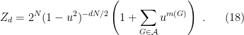
We can now express the 2-D Ising model’s partition function as

$\displaystyle Z= 2^N (1-u^2)^{-N} \prod_{[p]} (1+W(p)) ~. \ \ \ \ \ (31)$

6. Counting all the paths

We need to count paths, but we need to do the book-keeping of the signs. To track the signs, which count the windings of the tangent vector along the path, we will consider every “left turn” as ${1/4}$ sign change, so we will count a factor ${\alpha=e^{i \pi/4}}$ . Similarly for every “right turn” we will include a factor ${\bar \alpha = e^{- i \pi /4}}$ . For no turns, i.e. going straight, we will include no extra factor, or equivalently, a factor of 1. Finally, going backwards is forbidden, so for a turn of ${\pi}$ radians we will kill this possibility by using a factor of zero, 0.

Recall that the amplitude ${W(p)}$ of a path is just ${u}$ raised to the power of the length of the path, and with a sign equal to ${\pm 1}$ depending on how many times the tangent vector winds around the origin. Since the factors ${\alpha}$ can be used to keep track of the changes in the direction of the tangent vector, therefore the amplitude of any (non-periodic) path is simply equal to ${\bar \alpha^a \alpha ^b 1^c 0^d u^{a+b+c+d}}$ where ${a}$ is the number of right turns, ${b}$ is the number of left turns, ${c}$ is the number of no turns (i.e. straight ahead) and ${d=0}$ is the number of backwards or 180 degree turns, of which there are none since these are forbidden.

Since we know how to calculate amplitudes now for any particular path, let us now turn to the calculation of amplitudes for collection of paths. Following probability theory, wave mechanics or quantum mechanics, we will assume that amplitudes obey the principle of linear superposition. In other words, the combined amplitude for a collection of paths equals the sum of the amplitudes for each path.

We are first going to count all the paths that start and end at the origin, i.e. closed loops that go through the origin. We are going to calculate the path propagator, i.e. the amplitude for arriving at a site ${(x,y)}$ at step ${n}$ starting at the origin. The propagator has translation invariance, i.e. where we place the origin does not matter. We are going to ignore boundary conditions because boundary effects will disappear in the thermodynamic limit. We will always consider the directions in the order up, down, left, right, for convenience. Let the positive ${x}$ axis go towards the right and the positive ${y}$ axis go upwards. Let the amplitudes for arrival at a site going in the up, down, left and right directions be respectively ${U}$ , ${D}$ , ${L}$ and ${R}$ . These amplitudes can refer to either one single path or to a collection or “ensemble” of paths.

The amplitude ${U_n(x,y)}$ for arriving in the upwards direction (i.e., from below) at step ${n}$ at position ${(x,y)}$ is given by

$\displaystyle \begin{array}{rcl} {U_n(x,y) \over u} &=& U_{n-1}(x,y-1) + 0 D_{n-1}(x,y-1) \\ & & \quad + \alpha L_{n-1}(x,y-1) + \bar \alpha R_{n-1}(x,y-1) ~. \end{array}$

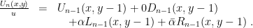
In words, this equation tells us that the amplitude to arrive going upwards at ${(x,y)}$ going upwards depends only on the amplitudes at step ${n-1}$ at position ${(x,y-1)}$ and on the turning factors ${\alpha}$ and ${\bar \alpha}$ , and on the factor ${u}$ of one bond.

Similarly, we thus have

$\displaystyle \begin{array}{rcl} {D_n(x,y) \over u} &=& 0 U_{n-1}(x,y+1) + D_{n-1}(x,y+1) \\ & & \quad + \bar \alpha L_{n-1}(x,y+1) + \alpha R_{n-1}(x,y+1) \\ {L_n(x,y) \over u} &=& \bar\alpha U_{n-1}(x-1,y) + \alpha D_{n-1}(x-1,y) \\ & & \quad + L_{n-1}(x-1,y) + 0 R_{n-1}(x-1,y) \\ {R_n(x,y) \over u} &=& \alpha U_{n-1}(x+1,y) + \bar\alpha D_{n-1} (x+1,y) \\ & & \quad + 0 L_{n-1} (x+1,y) + R_{n-1} (x+1,y) ~. \end{array}$

If a site ${(x,y)}$ can only be reached in ${m}$ steps with ${m>n}$ , then the amplitudes ${U_n(x,y)=D_n(x,y)=L_n(x,y)=R_n(x,y)=0}$ . This extension allows us to consider arbitrarily distant ${(x,y)}$ .

Before we calculate the amplitudes ${W(p)}$ of closed nonperiodic paths ${p}$ , which is what we need, let us first calculate the amplitudes of path segments. Consider all path segments that start at the origin and end at position ${(x,y)}$ after exactly ${n}$ steps. The total amplitude for this collection of path segments will be given by

$\displaystyle U_n(x,y)+D_n(x,y)+L_n(x,y)+R_n(x,y) ~ ,\ \ \ \ \ (32)$

which is just the sum of the amplitudes to end at ${(x,y)}$ coming in from each of the 4 possible directions.

We now have a situation where we can recursively express the amplitudes at step ${n}$ in terms of the amplitudes at step ${n-1}$ , however the recursion relations include a shift of the coordinates ${(x,y)}$ to a neighboring site. For example the amplitude ${U_n(x,y)}$ depends on the amplitudes at step ${n-1}$ at position ${(x,y-1)}$ rather than ${(x,y)}$ , and so forth. These translations pose a difficulty that we need to overcome.

We will now invoke the magical powers of the Fourier transform! This integral transform has many amazing properties. For example, convolutions become products and vice versa under Fourier transformation. Similarly, differential operators transform to simple algebraic multipliers. The particular property of the Fourier transform that we will use is the ability to convert translations into phase shifts. I use the term Fourier transform in the general sense, which includes Fourier series. The Dirac comb can be used to treat them both as part of a single theory. So let us define the Fourier transform ${\widehat U_n(k_x)}$ of ${U_n(x)}$ and the inverse transform as follows:

$\displaystyle \begin{array}{rcl} \widehat U_n(k_x,k_y)&=& \displaystyle\sum_{x=-\infty}^\infty \displaystyle\sum_{y=-\infty}^\infty U_n(x,y) e^{-ik_x x -k_y y} \\ U_n(x,y) &=& \displaystyle {1\over {(2\pi)^2}} \displaystyle\int_{0}^{2\pi} \displaystyle\int_{0}^{2\pi} \widehat U_n(k_x,k_y) e^{ik_x x +k_y y} ~dk_x dk_y ~ . \end{array}$

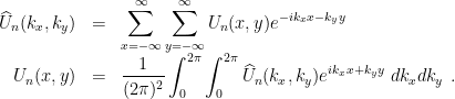
Are these quantities well defined? The Fourier transform is well defined for any ${L^1}$ function. Since for fixed ${n}$ the amplitude ${U_n}$ has compact support and is finite, therefore it lies in the space ${\ell^1(\Bbb Z)}$ of absolutely summable functions. However, it is possible for ${\widehat U}$ not to be an ${L^1}$ function! This topic is beyond the scope of this article. Suffice it to say that, in some sense, the inverse transform can also be made well defined even for non- ${L^1}$ functions.

Let us now explicitly calculate ${\widehat U}$ :

$\displaystyle \begin{array}{rcl} \widehat U_n(k_x,k_y) &=& \displaystyle\sum_{x=-\infty}^\infty \displaystyle\sum_{y=-\infty}^\infty e^{-ik_xx -k_yy} \bigg[ U_{n-1}(x,y-1) \\ & & \quad + 0 D_{n-1}(x,y-1) + \alpha L_{n-1}(x,y-1) + \bar \alpha R_{n-1}(x,y-1) \bigg] \\ &=& \displaystyle\sum_{x=-\infty}^\infty \displaystyle\sum_{y=-\infty}^\infty e^{-ik_xx -k_y(y+1)} \bigg[ U_{n-1}(x,y) \\ & & \quad + 0 D_{n-1}(x,y) + \alpha L_{n-1}(x,y) + \bar \alpha R_{n-1}(x,y) \bigg] \\ & =& e^{-i k_y} \bigg[ \widehat U_{n-1}(k_x,k_y) + 0 \widehat D_{n-1} (k_x,k_y) \\ & & \quad + \alpha \widehat L_{n-1} (k_x,k_y) + \bar \alpha \widehat R_{n-1} (k_x,k_y) \bigg] ~. \end{array}$

Note that the translation has disappeared and instead become a phase shift. For the transforms of the other amplitudes, we will get analogous expressions. Specifically, if we let ${v=e^{-i k_y}}$ and ${h=e^{+ik_x}}$ we can summarize the recursion relations for the transformed amplitudes as

$\displaystyle \begin{array}{rcl} \widehat U_n &=& u( v U_{n-1} + 0 \widehat D_{n-1} + v \alpha \widehat L_{n-1} + v \bar \alpha \widehat R_{n-1} ) \\ \widehat D_n &=& u( 0 U_{n-1} + \bar v \widehat D_{n-1} + \bar v \bar \alpha \widehat L_{n-1} + \bar v \alpha \widehat R_{n-1} )\\ \widehat L_n &=& u( \bar h \bar \alpha U_{n-1} + \bar h \alpha \widehat D_{n-1} + \bar h \widehat L_{n-1} +0 \widehat R_{n-1} )\\ \widehat R_n &=& u( h \alpha U_{n-1} + h \bar \alpha \widehat D_{n-1} + 0 \widehat L_{n-1} +h \widehat R_{n-1} )~.\\ \end{array}$

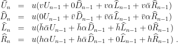
Notice that the Fourier transformed amplitudes for step ${n}$ are linear in the transformed amplitudes for step ${n-1}$ . So we can use the tools of linear algebra on this set of 4 equations. So let us define the vector

$\displaystyle \psi_n = \left[ \begin{array}{c} \widehat U_n\\ \widehat D_n \\ \widehat L_n \\ \widehat R_n \end{array} \right] ~. \ \ \ \ \ (33)$

and the matrix

$\displaystyle M = \left[ \begin{array}{cccc} v & 0 & v\alpha & v\bar \alpha\\ 0 & \bar v & \bar v \bar \alpha & \bar v \alpha \\ \bar h \bar \alpha & \bar h \alpha & \bar h & 0 \\ h \alpha & h \bar \alpha & 0 & h \end{array} \right] ~. \ \ \ \ \ (34)$

So we can express the recursion relation in matrix form as

$\displaystyle \psi_n = u M \psi_{n-1} ~, \ \ \ \ \ (35)$

which is much more concise than the 4 separate equations in 4 variables. Even better, we can iterate the recursion to obtain

$\displaystyle \psi_n = u^n M^n \psi_0 \ \ \ \ \ (36)$

where ${\psi_0}$ is the Fourier transformed amplitude for a loop of length zero, for arriving at the origin before the first step. But do we know which way the walk arrived at the origin? In general we do not know, but for loops, i.e. closed paths, we do! The ${\psi_0}$ for arriving at the origin is simply ${\psi_n}$ , because the path is a closed loop. From now on, we focus exclusively on loops. In the case of a loop, the way that the path started at the origin is identical to the way it ends at the origin.

Paths starting at the origin can only start in 4 possible directions. Let ${\epsilon _i}$ for ${i=1,2,3,4}$ be the basis unit vectors for the space of the ${\psi}$ for the directions up, down, left and right. Then the paths ending at the origin going upwards at the origin have total (Fourier transformed) amplitude ${ u^n \psi_0^T M^n \psi_0}$ with ${\psi=\epsilon_1}$ , and similarly for the other 3 directions. Here ${\epsilon^T}$ is the transpose of ${\epsilon}$ . So the total amplitude for all loops going through the origin is given by

$\displaystyle \displaystyle\sum _{i=1}^4 \epsilon_i ^T (uM)^n \epsilon_i ~. \ \ \ \ \ (37)$

For those familiar with Dirac’s bra-ket notation, we could write instead

$\displaystyle \displaystyle\sum _{i=1}^4 \langle {\epsilon_i|(uM)^n|\epsilon_i}\rangle ~, \ \ \ \ \ (38)$

however, we will stick with the usual linear algebra notation. The sum of the diagonal terms of a matrix is the trace, so we can rewrite the total amplitude for loops of length ${n}$ that end at the origin more concisely as,

$\displaystyle {\rm Tr~} (uM)^n ~. \ \ \ \ \ (39)$

We have been working with the Fourier transform ${\psi}$ of the amplitudes , so we need to inverse Fourier transform and evaluate the inverse transformed quantity at the origin, ${x=y=0}$ :

$\displaystyle {1\over (2\pi)^2 } \displaystyle\int_0^{2\pi} \displaystyle\int_0^{2\pi} {\rm Tr~} (uM)^n ~dk_x dk_y ~. \ \ \ \ \ (40)$

This expression is still not the correct amplitude because the sign of the amplitude is ${-1}$ times the number of times that the tangent vector of the path winds around the origin, so we must multiply by ${-1}$ . We have also only considered paths that end at the origin. If we have ${N}$ sites, then there are ${N}$ times as many paths. We have also counted each path twice: one in the “forward” direction and one in the “reverse” direction. So we have counted paths as well as their inversions. Multiplying by ${-1}$ and ${N/2}$ we get the total amplitude of closed paths of length ${n}$ :

$\displaystyle \displaystyle\sum_{p(n)} W(p)= - {N \over 2} {1\over (2\pi)^2 } \displaystyle\int_0^{2\pi} \displaystyle\int_0^{2\pi} {\rm Tr~} (uM)^n ~dk_x dk_y ~. \ \ \ \ \ (41)$

This expression includes all closed paths that start anywhere. But there are ${n}$ possible starting positions for a loop of length ${n}$ . So we are over-counting the total number of loops. If we quotient out the ${n}$ circular permutations, we get the correct final amplitude. Summing over ${n}$ , we get the total amplitude for all (non-equivalent) closed paths:

$\displaystyle \begin{array}{rcl} \displaystyle\sum_{n=1}^\infty {1\over n} \displaystyle\sum_{p(n)} W(p) &=& \displaystyle\sum_{n=1}^\infty - \displaystyle {N \over 2} \displaystyle {1 \over n} \displaystyle {1\over (2\pi)^2 } \displaystyle\int_0^{2\pi} \displaystyle\int_0^{2\pi} {\rm Tr~} (uM)^n ~dk_x dk_y \\ &=& \displaystyle {N \over 2} \displaystyle {1\over (2\pi)^2 } \displaystyle\int_0^{2\pi} \displaystyle\int_0^{2\pi} {\rm Tr~} \displaystyle\sum_{n=1}^\infty -\displaystyle{(uM)^n \over n} ~dk_x dk_y \\ &=& \displaystyle {N \over 2} \displaystyle{1\over (2\pi)^2 } \displaystyle\int_0^{2\pi} \displaystyle\int_0^{2\pi} {\rm Tr~} \ln (1-uM) ~dk_x dk_y ~. \end{array}$

Interchanging of the summation and integration is allowed provided we have absolute convergence. Similarly, for the logarithm we need to ensure that we have convergent power series. Let us take a closer look. The matrix ${M}$ has no element larger than 1. So the maximum trace of ${M}$ is 4 and the maximum trace of ${uM}$ is also 4. Hence, for ${|u|<1/4}$ the sum of the double integral is absolutely convergent and we can take the sum inside the integral. Next, let us look at the convergence of the sum, taken inside the trace inside the double integral. The summand is a matrix, so we have a matrix valued power series. If we consider the power series expansion for the logarithm of a matrix, then as usual the radius of convergence is for matrix norm (smaller than) 1. ${M}$ and ${uM}$ have norms no larger than 4. So for ${|u|<1/4}$ the power series converges in norm and we can express it as a logarithm. However, note that for the logarithm we do not in fact have to worry about convergence of the power series of the logarithm if we think in terms of formal power series or analytic continuation beyond the branch point singularity. For example, it is well known that the Riemann zeta ${\zeta(z)}$ function defined as a power series does not converge for small positive or negative real part of ${z}$ , but analytic continuation (or equivalent methods) allow it to be uniquely defined beyond the radius of convergence. Similarly, the formal power series of the logarithm is well defined independently of convergence (i.e. well defined algebraically rather than analytically).

We thus have an expression for the amplitudes that includes all non-periodic paths, up to equivalence under inversions and circular permutations. But what about periodic paths? A periodic path of total length ${n}$ with period ${w}$ has ${n/w}$ starting points only, not ${n}$ . So the above expression counts all non-periodic paths with weight 1 but also periodic paths with weight ${1/w}$ . What about the sign of periodic paths? The sign is ${(-1)^{w-1} }$ because the sign of a periodic path is defined as ${-(-1)^{wt}=(-1)^{wt+1}}$ , see Eq. (22). So for even period, the sign for terms of order ${W^w}$ is is always ${-1}$ , whereas for odd period the sign should be the same as for the nonperiodic path, i.e. ${W}$ .

Let ${[p]}$ again denote the equivalence class of non-periodic paths, with inversions and circular permutations considered equivalent. We can then write

$\displaystyle \begin{array}{rcl} \displaystyle\sum_{n=1}^\infty \displaystyle {1\over n} \displaystyle\sum_{p(n)} W(p)&=& \displaystyle\sum_{[p]} \left(W-{W^2\over2} + {W^3 \over 3}-\ldots\right) \\ &=& \displaystyle\sum_{[p]} \ln (1+W) \\ &=& \ln \displaystyle\prod_{[p]} (1+W) ~ . \end{array}$

Note that the sign for even period is negative, but the sign of ${W^w}$ for odd ${w}$ is the same as the sign of ${W}$ . (Again, for readers concerned about convergence, since ${|W|<1}$ , the series for ${\ln (1+W) }$ converges absolutely.)

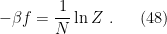
Substituting these last few results back into (17) we thus get

$\displaystyle Z = 2^N (1-u^2 )^{-N} \exp \left[ \displaystyle{N\over 2 (2\pi)^2 } \displaystyle\int_0^{2\pi} \displaystyle\int_0^{2\pi} {\rm Tr~} \ln (1-uM) ~dk_x dk_y \right] ~. \ \ \ \ \ (42)$

To proceed further, we must calculate the trace of the log of ${1-uM}$ . But this is actually quite easy, because the sum of logarithms is the logarithm of the products. In this case, the relevant sum and product are of the eigenvalues of ${1-uM}$ . Specifically, ${{\rm Tr~} \ln (1-uM) = \ln \det ( 1-uM)}$ , so

$\displaystyle Z = 2^N (1-u^2 )^{-N} \exp \left[ \displaystyle{N\over 2 (2\pi)^2 } \displaystyle\int_0^{2\pi} \displaystyle\int_0^{2\pi} \ln \det (1-uM) ~dk_x dk_y \right] ~. \ \ \ \ \ (43)$

The determinant can be found using methods such as expansion in minors, Laplace expansion or Leibniz’ formula. We obtain the value

$\displaystyle \det (1-uM ) = (u^2+1)^2 + 2u(u^2-1) (\cos (k_x) + \cos(k_y)) ~. \ \ \ \ \ (44)$

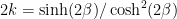
Let us try to simplify this expression. Recall that ${u=\tanh(\beta)}$ so that

$\displaystyle \begin{array}{rcl} 1-u^2&=& \displaystyle { 1\over \cosh^2 (\beta) } \\ \sinh (2\beta) &=& 2 \sinh (\beta) \cosh(\beta)\\ &=& 2 u \cosh^2(\beta)\\ \cosh(2\beta)&=& \displaystyle { \cosh^2(\beta) + \sinh^2(\beta) \over \cosh^2(\beta) - \sinh^2(\beta) } \\ &=& \displaystyle { 1 + u^2 \over 1- u^2 } \end{array}$

so that

$\displaystyle \begin{array}{rcl} (u^2+1)^2&=& \displaystyle { \cosh^2(2\beta)\over \cosh^4(\beta) } \\ 2u(u^2-1)&=& - \displaystyle { \sinh(2\beta)\over \cosh^4(\beta) } ~. \end{array}$

Substituting back, we obtain

$\displaystyle \det (1-uM ) = \displaystyle { \cosh^2(2\beta)- \sinh(2\beta)(\cos (k_x) + \cos(k_y)) \over \cosh^4(\beta) } ~, \ \ \ \ \ (45)$

and

$\displaystyle \ln \det ( 1-uM) = -4 \ln \cosh(\beta) + \ln \left[\cosh^2(2\beta)-\sinh(2\beta)(\cos(k_x) + \cos(k_y)) \right] ~.\ \ \ \ \ (46)$

We are now essentially done and can easily obtain the solution found by Onsager. The Helmholtz free energy ${F}$ is defined according to

$\displaystyle -\beta F = \ln Z \ \ \ \ \ (47)$

and the free energy per particle ${f=F/N}$ is thus given by

$\displaystyle -\beta f = {1\over N} \ln Z ~. \ \ \ \ \ (48)$

Following Onsager, let us define ${\ln \lambda=-\beta f}$ , i.e. the partition function per spin.

Substituting, we get

$\displaystyle \begin{array}{rcl} &\ln \lambda=& \displaystyle{1\over N} \bigg[ N \ln 2 + 2N \ln \cosh(\beta) \\ & & \quad + \displaystyle{N\over 8 \pi^2} \displaystyle\int_0^{2\pi} \displaystyle\int_0^{2\pi} \bigg( -4 \ln \cosh(\beta) \\ & & \quad \quad + \ln \left[\cosh^2(2\beta)-\sinh(2\beta)(\cos(k_x) + \cos(k_y)) \right]\bigg) dk_x dk_y \bigg] \\ &=& \ln 2\! + \displaystyle{1\over 8 \pi^2} \displaystyle\int_0^{2\pi} \displaystyle\int_0^{2\pi} \ln \big[\cosh^2(2\beta)-\sinh(2\beta)(\cos(k_x) + \cos(k_y)) \big] dk_x dk_y ~~~~~~~~~ \\ ~ \\ &=& \ln [2 \cosh(2\beta)] + \displaystyle{1\over 8 \pi^2} \displaystyle\int_0^{2\pi} \displaystyle\int_0^{2\pi} \ln \big[1-{2k }(\cos(k_x) + \cos(k_y)) \big] dk_x dk_y \nonumber \\ &=& \ln [2 \cosh(2\beta)] + \displaystyle{1\over 2 \pi^2} \displaystyle\int_0^{\pi} \displaystyle\int_0^{\pi} \ln \big[1-{2k }(\cos(k_x) + \cos(k_y)) \big] dk_x dk_y ~. \nonumber \\ \end{array}$

where ${2k = \sinh(2\beta)/\cosh^2(2\beta)}$ . We are done!

Specifically, the above result is equivalent to Onsager’s original expression. Except for notation, it is identical to Eq. (109b) of the 1944 paper, specialized to the case of unit symmetric coupling ${J=1}$ for both directions. It is also essentially the same as Eq. (5.29) in Feynman’s book [3].

7. The hypergeometric series for the partition function

I originally went through the above exercise with the sole motivation of wanting to understand Onsager’s solution. Quite by accident, however, I unexpectedly stumbled onto a very nice result about the 2-D Ising model.

Onsager’s solution above is written in terms of a definite integral. No “closed form” expression, even in terms of special functions, was generally known — until now! I recently uploaded to arXiv a paper in which I derive the hypergeometric series for the partition function. Hypergeometric series generalize the geometric series.

I was especially happy to learn that in the 1970s Larry Glasser and Lars Onsager had arrived at a result (unpublished) very similar to mine (see link to arXiv below for details). Their result and mine are related via a hypergeometric identity, which I hope to investigate more closely when time permits.

Here is the link to my paper on arXiv.

Notes

[1] L. Onsager, Phys. Rev. 65, 117 (1944).
[2] H. E. Stanley, Introduction to Phase Transitions and Critical Phenomena (Oxford University
Press, Oxford, New York, 1971).
[3] R. P. Feynman, Statistical Mechanics. A set of lectures (Benjamin and Cummings Publishing, Reading, 1972).
[4] B. McCoy and T. Wu, The two dimensional Ising model (Harvard University Press, Cambridge, 1973).
[5] K. Huang, Statistical Mechanics (John Wiley & Sons, New York, 1987).
[6] R. J. Baxter. Exactly solved models in statistical mechanics (Academic Press, London, 1989).
[7] S. G. Brush, Rev. Mod. Phys. 39, 883 (1967).
[8] G. F. Newell and E. W. Montroll, Rev. Mod. Phys. 25, 353 (1953).
[9] B. A. Cipra, The American Mathematical Monthly 94, 937 (1987).
[10] B. L. Van Der Waerden, Z. Physik 118, 473, 1941.
[11] M. Kac and J. C. Ward, Phys. Rev. 88, 1332, 1952.
[12] S. Sherman, J. Math. Phys. 1, 202 (1960).
[13] G. A. T. F. da Costa and A. L. Maciel, Rev. Bras. Ensino de Física 25, 49 (2003).
[14] S. Salinas, Introduction to Statistical Physics (Springer, Berlin, 2001).

6 thoughts on “Onsager’s solution of the 2-D Ising model: The combinatorial method”

Pingback: Ising model resources | Sp1nor
Gandhi Viswanathan on 24/07/2015 at 17:24 said:

UPDATE: The paper on arXiv was recently published in JSTAT. Here is the link: http://dx.doi.org/10.1088/1742-5468/2015/07/P07004

Reply ↓
Pingback: Fermionization of the 2-D Ising model: The method of Schultz, Mattis and Lieb | Gandhi Viswanathan's Blog
Gandhi Viswanathan on 30/08/2021 at 16:24 said:

UPDATE: I recently published in JSTAT another paper on the hypergeometric formulation of the 2D Ising model. See here: https://arxiv.org/abs/2104.03430

Reply ↓
Alexander (Alex) Punnoose on 01/12/2022 at 22:48 said:

Thank you for a clear exposition of the combinatorics method. I was wondering if you have come across an extension of the same method to include periodic boundary conditions in two dimensions?

Reply ↓
- Gandhi Viswanathan on 02/12/2022 at 14:26 said:
  
  The treatment above actually is for the 2D model with periodic boundary conditions. See just before eq 10. As a general rule, if you see that the Fourier transform is being used, then most likely periodic B.C. are also being used, explicitly or implicitly. This is because the Fourier transform is most useful when the underlying problem has translation invariance. Periodic B.C. guarantee translation invariance. But if you use, say, open boundary conditions, then the boundary breaks translation invariance symmetry. Having said this, recall that in the thermodynamic limit, the boundary conditions become irrelevant for Hamiltonian systems with only short-range interactions, as is the case for the 2D ferromagnetic Ising mode with nearest neighbor interactions.
  
  Reply ↓

Gandhi Viswanathan's Blog

Physics, Math and Life as a Scientist

Onsager’s solution of the 2-D Ising model: The combinatorial method

6 thoughts on “Onsager’s solution of the 2-D Ising model: The combinatorial method”

Leave a reply to Gandhi Viswanathan Cancel reply

Share this:

Related

6 thoughts on “Onsager’s solution of the 2-D Ising model: The combinatorial method”

Leave a reply to Gandhi Viswanathan Cancel reply