Domain coloring for visualizing complex functions

The above figure shows a domain color plot for the function ${z\mapsto {1/(1 - i z )} -(1 + i z)}$ .

I have been relearning complex analysis and decided to have some fun plotting complex functions. It is easy to visualize graphically a real function ${f:\Bbb R\rightarrow \Bbb R}$ of a real variable. To visualize ${f(x)}$ , we can plot ${x}$ on the horizontal axis and ${y=f(x)}$ on the vertical axis, as we learn in high school mathematics. It is more difficult, however, to visualize the function ${g:\Bbb C\rightarrow \Bbb C}$ , because ${g}$ is a complex function of a complex variable. A complex number ${z}$ can be expressed in terms of real numbers $x, ~y$ as ${z=x+ i y}$ . To visualize the complex domain of a function, one thus requires 2 real dimensions. The complex function ${g(z)}$ must then be plotted on the remaining dimensions. If we lived in 4 dimensional space, it would be easy to plot a complex function of a complex variable. The problem is that we live in three dimensions, not four. Domain coloring is a method to overcome this limitation. The basic idea is to use colors and shades etc. as extra dimensions for visualizing functions.

I first heard about domain coloring when I came across Hans Lundmark’s complex analysis pages. For readers unfamiliar with domain coloring, I recommend reading up on it first. There is also a wikipedia article on the subject.

Introduction

The pictures below were generated using Wolfram’s Mathematica software (many thanks to my department colleague Professor Marcio Assolin). I adapted the code from the discussion on stackexchange here, and also here.

The first figure below shows the identity function ${f(z)=z}$ :

The horizontal axis is the real axis and the vertical the imaginary axis of the domain ${z}$ . The 29×29 grid is not deformed in this case because the identity function ${f(z)=z}$ does “nothing.” But I decided to include this example to illustrate how the colors and shades code information. First of all, notice that as we go around the origin ${z=0}$ , the colors go from red on the positive real line, to green on the positive imaginary axis, to cyan on the negative real axis, to purple on the negative imaginary axis and then back to red again.

The color represents the argument of the function. In this case, since we can write ${z=r e^{i\theta}}$ the argument ${\theta}$ wraps back around every time we turn ${2\pi}$ radians around the origin in the complex plane.

Note that in addition to color, there is shading. Notice that at ${|z|=1/2}$ , ${|z|=1}$ and ${|z|=2}$ there are discontinuities in shading. As we increase the absolute value of ${z}$ , the shading gets darker and discontinuously gets brighter and this process repeats itself. Indeed, the shading has been used to plot the absolute value of the function. Every time the absolute value doubles, the shading goes through one cycle, becoming discontinuously brighter.

Monomials

Let us now look at more complicated functions. The pictures below show the functions ${z\mapsto z^2}$ and ${z\mapsto z^3}$ .

Now, things look more interesting! The first thing to note is that the 29×29 grid is distorted. The grid shown is the inverse image of the grid of the identity map. So for the function defined by ${f(z)=z^2}$ , the procedure is as follows. Take the points of the grid and put them into some set ${S}$ . Then calculate the inverse image ${f^{-1}(S)}$ , i.e. the set of points that map to ${S}$ . This inverse image is the grid shown above.

Notice how the distorted grid seems to preserve right angles, except at the origin. Indeed, holomorphic functions are typically also conformal (i.e., angle preserving) in many instances, and we will return to this topic further below. At the origin, the monomial functions above are clearly not conformal.

Take a look at the colors. Instead of cyclying through the rainbow colors going once around the origin, the colors cycle 2 and 3 times, respectively, for ${z^2}$ and ${z^3}$ . This is easy to understand if we write ${z=re^{i \theta}}$ (for real ${r}$ and ${\theta}$ ), so that ${z^2=r^2 e^{2i\theta}}$ and ${z^3=r^3 e^{3i\theta}}$ . So ${z^2}$ and ${z^3}$ circle the origin 2 and 3 times every time ${z}$ goes around the origin once.

Finally, notice that the shading cycles through more quickly. Indeed, ${|z^2|}$ and ${|z^3|}$ double more quickly than ${|z|}$ .

Poles

The monomial functions above have zeroes, but no poles. What do poles look like? The image below shows the function ${z\mapsto 1/z}$ .

Notice how the colors cycle around “backwards.” Indeed, the argument of ${z}$ and ${z^{-1}}$ are negative of each other. Notice also how the shading now has discontinuities in the “opposite” sense (compare with ${z\mapsto z}$ in the first image above).

It is also worthwhile to look at the grid. The original grid of lines has transformed into a patchwork of circles. To show this more clearly, I modifed the image to show only a few grid lines, corresponding to real and imaginary lines at ${\pm 1,2,3,4,5}$ :

In the image above the grid lines are now clearly seen to have mapped into circles. In higher order poles, the colors cycle around (backwards) a number equal to the order of the pole. Here are poles of order 2 and 3, shown with only some grid lines for greater clarity:

In addition to poles, there are other kinds of singularities. Removable singularities are not too interesting, because basically a “point” is missing. If we “manually add” the point, the singularity is “removed” — hence the name.

In addition to removable singularities and poles, there are also what are known as essential singularities. Essential singularities can be thought of, loosely speaking, as poles of infinite order. Further below, we will take a look at essential singularities.

Now consider a function with a zero as well as a pole:

The function shown above is ${z\mapsto (z-1)+ 1/(z+1)}$ , which has a zero at ${z=0}$ and simple pole at ${z=-1}$ .

Non-holomorphic functions

Having looked at examples of holomorphic and meromorphic functions, let us look at more complicated non-holomorphic function. The figure below shows ${|z|}$ , the absolute value of ${z}$ .

The color is red because ${|z|}$ is always non-negative real. The grid is gone and we have circles instead: we do not have conformality. The Cauchy-Riemann equations are impossible to satisfy because ${|z|}$ is always real, the imaginary part being identically zero everywhere.

The complex conjugate function ${z\mapsto \bar z}$ also is not analytic. Here is ${z\mapsto \bar z}$ :

Notice that it looks just like the identity map, but reflected along the real axis. The imaginary axis is “backwards”. Still, angles are preserved, so why is this function not holomorphic? The answer is that the angle orientations are reversed, i.e. the function is antiholomorphic rather than holomorphic. The colors cycle around “backwards” in this case because the complex conjugate of $r e^{i \theta}$ is $r e ^{- i \theta}.$ Conformal maps preserve oriented angles, rather than just angles. Indeed, the complex conjugate function is neither holomorphic nor conformal.

The exponential function and its Taylor polynomials

Let us now look at a transcendental holomorphic function: the exponential function ${z\mapsto \exp(z)}$ . The images below show the exponential function at two scales.

Notice that the colors now cycle through going up and down vertically. The reason for this is as follows. If we write ${z=x + i y }$ , then

$\exp[z]=e^{x+i y } = e^x e^{i y} ~.\ \ \ \ \$

So ${y}$ , which is the imaginary part of ${z}$ , determines the argument, hence the color. The zoomed out version makes it clear that the argument is periodic with period ${2 \pi}$ in the imaginary direction.

While on the topic of the exponential function, let us take a look at Talyor polynomial expansions. The figure below shows the Talor polynomial of degree 5.

Notice the 5 zeroes, which lie on an arc like the letter “C” slightly to the left of the origin. The exponential function does not have zeroes, of course. We know that if we take the infinite degree Talyor polynomial, i.e. the infinite Taylor series expansion, then we recover the exponential function. We can already see that for positive real part and small imaginary part of ${z}$ , the Taylor polymial above is starting to behave qualitatively like the exponential function.

Essential singularities

Having seen the exponential function, we can now look at essential singularities. Observe that the Laurent expansion of ${\exp(1/z)}$ around the origin in ${z}$ has an infinite number of terms of negative power in ${z}$ . The singularity at the origin is thus stronger than a pole of any finite order. The figure below shows ${z\mapsto \exp(1/z)}$ , shown at three different scales. The third figure is a zoom of the second, which is a zoom of the first.

The software is apparently having some trouble near the origin, in the last figure! The reason for this is the Great Picard’s theorem, which says, loosely speaking, that an analytic function near an essential singularity takes all possible complex values, with at most 1 exception. In the case of ${z\mapsto \exp(1/z)}$ , the function cannot become zero, which is the exceptional value. As we approach the origin, the argument (i.e. color) changes, cycles around, etc., increasingly quickly.

Let us now look at some trigonometric functions:

${\sin(z)}$ :

${\tan(z)}$

We can clearly see the zeroes in ${\sin(z)}$ and the poles and zeroes of ${\tan(z)}$ . Moreover, it is clear that these are periodic functions.

Compare the above trigonometric functions with their inverses:

${\arcsin(z)}$

${\arctan(z)}$

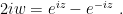
Notice that on the real line, for ${|z|>1}$ there is a discontinuity in color for arcsine. Similarly, for arctan there is a color discontinuity on the imaginary axis. To understand this jump in color, recall that ${|\sin(x)|\leq 1}$ , which means that the inverse function ${\sin^{-1}(x)=\arcsin(x) }$ is not defined for ${x}$ outside the interval ${ -1\leq x\leq 1}$ . Recall also that ${\sin(x)=\sin(x+2\pi)}$ , so that the inverse function ${\sin^{-1}}$ must be multivalued. What is being shown above is the principal branch.

It helps to switch over to the logarithmic form. Recall that

$\displaystyle \sin(z)= {e^{iz} - e^{-iz} \over 2i } ~. \ \ \ \ \$

If we write ${z=\arcsin(w)}$ , then ${\sin(z)=w}$ . Substituting, we get

$\displaystyle 2iw ={e^{iz} - e^{-iz} }~. \ \ \ \ \$

To simplify the algebra, let ${e^{iz}=Z}$ , so that

$\displaystyle 2iw = {Z - Z^{-1} } ~, \ \ \ \ \$

which gives us a quadratic equation:

$\displaystyle Z^2 -2iwz -1 =0~, \ \ \ \ \$

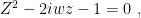
whose roots are

$\displaystyle Z= iw \pm \sqrt{1-w^2} ~. \ \ \ \ \$

So we finally get

$\displaystyle z=\arcsin(w)=-i \log Z= -i \log\left( iw \pm \sqrt{1-w^2} \right) ~. \ \ \ \ \$

So the branch cut in the ${\arcsin}$ function is due to the 2 possible values of the square root. There is a branch point at ${w=\pm 1}$ and there is actually another branch point at infinity.

Branch points and cuts

Let us look at branch points more closely. As we know, the square root is multivalued, and the figure below shows the two branches, with the principal branch at the bottom.

Note how in each branch alone the colors do not cycle all the way through the rainbow colors. The missing colors of one branch are on the other branch. To see both branches, one would need to visualize the Riemann surface for the square root, a topic beyong what I wish to cover here.

The figure below shows the 3 branches of the cube root function, with the principal branch at the top:

There is more than 1 type of branch point. Algebraic branch points are those that arise from taking square roots, cubic roots, and ${n}$ -th roots (for positive integer ${n}$ ). In general there will be ${n}$ well defined branches.

What happens if one takes ${n}$ to be a positive irrational number? Here is a hint:

$z^{\alpha} = e^{\alpha \ln z} ~.$

If we choose ${\alpha}$ rational, say ${\alpha=p/q}$ , then putting ${z=r e^{i\theta + 2n\pi i}}$ we get ${\ln z= \ln r + i\theta + 2n\pi i}$ , so that

$\displaystyle z^\alpha = r^{p/q} e^{i \alpha \theta} e^{ 2\pi i (np /q)} ~.$

But ${n p/q}$ is rational, and so there can be at most ${q}$ branches. But if ${\alpha}$ is irrational, this argument does not work. Instead of ${np/q}$ we get ${n\alpha}$ , which can never equal an integer. So the branches never cycle through and the number of branches is infinite. Indeed, the logarithm above leads to a infinite branching, as we will see below.

There is a more complicated type of branch point in the function ${z\mapsto \exp(1/z^{1/n})}$ for integer ${n}$ . If we loop around the origin ${n}$ times, the function returns to the original starting point (i.e. there is finite monodromy). However, there is an essential singularity at the origin. In other words, there is the unhappy coincidence of the algebraic branch point of ${1/z^{1/n}}$ sitting exactly on top of an essential singularity. Such branch points are known as transcendental branch points.

The figure above shows ${z\mapsto \exp(1/z^{1/2} )}$ . The essential singularity coincides with the branch point.

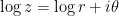
Finally, as we saw above, there are branch points where the number of branches is infinite. Consider the complex logarithm. If we again write ${z=r e^{i \theta}}$ then ${\log z= \log r + i \theta}$ . Since ${\theta}$ and ${\theta \pm 2\pi}$ give same value of ${z}$ , the logarithm is multivalued. The branch cut is usually taken at ${\theta=\pm \pi}$ . Here is the logarithm:

The zero at ${z=1}$ is clearly visible, as is the branch cut along the negative real axis.

The complex logarithm, like other multivalued functions, could instead be visualized as Riemann surfaces. Here is an example of the Riemann surface of the complex logarithm.

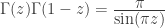
Euler’s reflection formula

Let us next consider another topic related to Weierstrass’s beautiful factorization theorem, which states that every entire function can be expressed as an infinite product. Among the best known infinite products are the one used by Euler to solve the Basel problem, and the product formula for Euler’s gamma function. Indeed, the gamma function is, in a sense, one half of the sine function (or cosecant). Put differently, the sine function is the product of two gamma functions:

$\Gamma(z)\Gamma(1-z) = {\displaystyle \pi \over \displaystyle \sin (\pi z) }$ .

Proofs can be found in textbooks. Here I wish to focus on the zeroes and poles. Take a look at these figures:

The figures above show ${1/\Gamma(z)}$ and ${1/ [\Gamma(z)\Gamma(1-z) ]}$ . Note the zeroes at the non-positive integers in the first image, correponding to the poles of the gamma function. If we multiply two gamma functions, so that there are zeroes at all integers, we basically get ${\sin(2\pi z)}$ upto a constant! Indeed, the last figure above is identical, up to scale, to that of the sine function seen earlier.

When are holomorphic functions conformal?

Finally, let us take a closer look at conformality, i.e. the angle-ṕreserving property found in many holomorphic functions. The examples above of monomials of degree greater than 1 and poles shows clearly that conformality can break down at zeroes and poles.

Consider again the function ${z \mapsto z^2}$ below:

Conformality indeed breaks down at the zero at the origin, as expected.

But if a function is holomorphic with no zeroes in a region, is it necessarily conformal in that region? The answer is NO, as seen from the following counter-example:

${z \mapsto z^2+1}$

There is no zero at the origin, yet conformality breaks down!

To understand why, recall that to preserve angles, the map must locally be a scaled rotation (upto a translation). So the Jacobian determinant of the conformal map must be some positive constant. It is easy to show that the Cauchy-Riemman equations lead to a scaled rotation, provided the derivative is not zero. If the derivative is zero, however, the function need no longer be a scaled rotation, so angles need not be preserved.

In the example above, the function is holomorphic at the origin, but the derivative is zero at the origin, in other words, the origin is a critical point. Moreover, as ${z}$ moves around the origin once, the function ${z^2+1}$ moves around 1 twice, hence the breakdown in conformality.

Conversely, if a holomorphic function has a critical point at the origin, then its Taylor series does not contain a term of degree 1. But all higher order monomials ${z^n}$ break the conformal property at the origin, so the function cannot be conformal at the critical point. By translating arbitrary functions such that a critical point is on the origin, we can understand the following well known result:

A holomorphic function is conformal if and only if there are no critical points in the region of interest.

NOTES:

[1]. Below is the Mathematica code I used for the plot of the identity map. The code has been adapted from the discussion on stackexchange here and also here.

f[z_] := z;

paint[z_] :=
Module[{x = Re[z], y = Im[z]},
color = Hue[Rescale[ArcTan[-x, -y], {-Pi, Pi}]];
shade = Mod[Log[2, Abs[x + I y]], 1];
Darker[color, shade/4]];

ParametricPlot[{x, y}, {x, -3, 3}, {y, -3, 3},
ColorFunctionScaling -> False,
ColorFunction -> Function[{x, y}, paint[f[x + y I]]], Frame -> True,
MaxRecursion -> 1, PlotPoints -> 300, PlotRangePadding -> 0,
Axes -> False , Mesh -> 29,
MeshFunctions -> {(Re@f[#1 + I #2] &), (Im@f[#1 + I #2] &)},
PlotRangePadding -> 0, MeshStyle -> Opacity[0.3], ImageSize -> 400]

4 thoughts on “Domain coloring for visualizing complex functions”

theblogbyablob on 09/10/2014 at 06:13 said:

Dear Gandhi, this is quite fascinating. It gives me some insight into a study that I am now doing. I shall email you with questions for guidance.

Reply ↓
Janilo on 09/10/2014 at 09:21 said:

A very useful toolkit for those who are lecturing complex functions or even for researchers in Field Theory, Astrophysics, and many other branches of Physics.

Reply ↓
Pingback: The Aperiodical
Pingback: DOMAIN COLORING | Éric Carvalho Rocha

Gandhi Viswanathan's Blog

Physics, Math and Life as a Scientist

Domain coloring for visualizing complex functions

Introduction

Monomials

Poles

Non-holomorphic functions

The exponential function and its Taylor polynomials

Essential singularities

Branch points and cuts

Euler’s reflection formula

When are holomorphic functions conformal?

4 thoughts on “Domain coloring for visualizing complex functions”

Leave a comment Cancel reply

Introduction

Monomials

Poles

Non-holomorphic functions

The exponential function and its Taylor polynomials

Essential singularities

Branch points and cuts

Euler’s reflection formula

When are holomorphic functions conformal?

Share this:

Related

4 thoughts on “Domain coloring for visualizing complex functions”

Leave a comment Cancel reply