Berezin’s 1969 solution of the 2D Ising model

In other blog articles I have previously mentioned my fascination with the Ising model and Onsager’s seminal solution of the 2D problem. I have also previously opined that, of all methods of solution, I consider the Grassmann algebraic method based on fermionic path integration (Berezin integration) to be the most elegant.

My first contact with the Grassmann variable method was via the seminal trilogy papers of Samuel dating from 1980. I was also familiar with the work of Polyakov and Dotsenko from a few years before that on the continuum Ising model.

However, I was almost shocked to find out that Felix Berezin himself gave a solution to the 2D Ising model — one decade before, in 1969!  I thank Massimo Ostili for bringing to my attention the original paper by Berezin. (It appears to me that, perhaps, credit and priority for original works are still ongoing issues that remain to be satisfactorily dealt with in the science community.) I found the original work of Berezin to be highly pleasurable to read.  For those unfamiliar with the work of this renowned physicist, credit goes to Berezin for modifying Feynman’s “bosonic” path integral formulation of quantum mechanics so that it could be applied to fermions.   These advances naturally led to supersymmetry and to supermathematics.  It would not be an exaggeration to claim that Berezin was one of the greatest physicists of the 20th century. Those interested to know about Berezin are referred to the book chapter by Robert Minlos.

You can find a PDF copy of the paper here. Enjoy!

Internal energy of the 2D Ising model

The above domain coloring plot shows an analytic continuation to the complex plane of the internal energy of the 2D Ising model. The domain variable is , which is a standard high temperature variable used to study the 2D Ising model.

I originally made the plot in 2014 soon after I first began to study the exact solution of the Ising model. A few days ago, I happened to find this old picture from 2014 and decided to share it here.

What a beautiful model! I had forgotten just how beautiful the structure is.

The 2 circles represent thermodynamic limit of the zeroes of the partition function. In this limit, singularities appear where the zeroes would be, as can be seen from Onsager’s formula. The critical temperature of the Ising model corresponds to the singularities on the real line, of which there are 4. The two singularities closer to the origin on the real line give the well known positive and negative critical temperatures . The other two give physically non-realizable complex critical temperatures, which are related to the standard critical temperatures via a symmetry known as the inversion relation (see MT Jaekel and JM Maillard, Symmetry relations in exactly soluble models, Journal of Physics A: Mathematical and General, 1982).

---

Mathematica Code:

f[z_] := (-\[Pi] (1 + z^2)^2 +
2 (1 – 6 z^2 + z^4) EllipticK[(16 z^2 (-1 + z^2)^2)/(1 + z^2)^4])/(
2 \[Pi] (z + z^3));

paint[z_] :=
Module[{x = Re[z], y = Im[z]},
color = Hue[Rescale[ArcTan[-x, -y], {-Pi, Pi}]];
shade = Mod[Log[2, Abs[x + I y]], 1];
Darker[color, shade/4]];

ParametricPlot[{x, y}, {x, -3, 3}, {y, -3, 3},
ColorFunctionScaling -> False,
ColorFunction -> Function[{x, y}, paint[f[x + y I]]], Frame -> True,
MaxRecursion -> 1, PlotPoints -> 300, PlotRangePadding -> 0,
Axes -> False , Mesh -> 29 , Mesh -> {Range[-5, 5], Range[-5, 5]},
MeshFunctions -> {(Re@f[#1 + I #2] &), (Im@f[#1 + I #2] &)},
PlotRangePadding -> 0, MeshStyle -> Opacity[0.3], ImageSize -> 400]

Exact solution of the 2D Ising model via Grassmann variables

1. Introduction

In 1980 Stuart Samuel gave what I consider to be one of the most elegant exact solutions of the 2D Ising model. He used Grassmann variables to formulate the problem in terms of a free-fermion model, via the fermionic path integral approach. The relevant Grassmann action is quadratic, so that the solution can be found via well-known formulas for Gaussian integrals.

In previous articles, I derived Onsager’s celebrated expression for the partition function of the 2D Ising model, using two different methods. First, I used a combinatorial method of graph counting that exploits the theory of random walks (see here). In the second article (see here), I reviewed the method of Schultz, Mattis and Lieb of treating the 2D Ising model as a problem of many fermions. Here I further explore the connection between the Ising model and fermions.

This article is based on my study notes. I more or less have followed Samuel’s solution of the 2D Ising model using Grassmann variables, but I had expanded the calculations for my own convenience.

Whereas on the one hand the behavior of bosons can be described using standard path integrals, known as bosonic path integrals, on the other hand the path integral formulation for fermions requires the use of Grassmann variables. Grassmann numbers can be integrated, but not using the standard approach based on Riemann sums and Lebesgue integrals, etc. Instead, they must be integrated using Berezin integration. I have previously written about Grassmann variables and Berezin integrals here.

In what follows, I assume familiarity with the 2D Ising model. Readers who find it difficult to understand the details are referred to the two previously mentioned articles, which are introductory and easier to understand.

The partition function can be approached as a power series either in a high temperature variable or a low temperature one. Consider first the high temperature expansion. It is well known that the partition function of the 2D Ising model is proportional to the generating function of connected or disconnected graphs in which all nodes have even degree, and edges link only nearest neighbors on the infinite square lattice. Graph nodes correspond to sites and links correspond to bonds. In such graphs, every incoming bond at a site has at least one corresponding outgoing bond, because each site has an even number of bonds. To each such “closed graph,” there are corresponding directed graphs, where the links are directed. Since each bond appears at most once in any such directed graph, but never twice or more, we can enumerate such closed directed graphs by assigning pairs of Grassmann variables to each bond. In this case, the generating function, when evaluated in a suitable high temperature variable (such as ), gives the Ising model partition function up to a known prefactor.

Here, I do not use the above high temperature expansion, in terms of loops or multipolygons. Instead, I use a low temperature expansion and enumerate non-overlapping magnetic domains, following Samuel’s original work. Specifically, each configuration of the Ising model corresponds to a specific domain wall configuration. So summing over all domain wall configurations is equivalent to a sum over all spin states, excepting for a 2-fold degeneracy since each domain wall configuration corresponds to 2 possible spin configurations.

Since the Ising model on the square lattice is self-dual, the high temperature approach using overlapping multipolygons and the low temperature appproach using non-overlapping multipolygons on the dual lattice are equivalent, of course. Either way, explicit evaluation of a Berezin integral gives the exact solution. Specifically, we assign 4 Grassmann variables to each site of the dual lattice. Equivalently, one can instead think as follows: there are two types of Bloch walls, “vertical” domain walls and “horizontal” walls and each wall segment has two ends. A Bloch wall can thus be represented by Grassmann variables at 2 different sites. A corner of a Bloch domain can be represented by matching a vertical and horizontal variable at a single site. Finally, so-called “monomer” terms consist of 2 horizontal or 2 vertical variables. They represent the absence of a corresponding bond, and also of corners. A single monomer term at a site represents a domain wall that goes straight through a site, but perpendicularly to the monomer and without going around a corner. Two monomer terms at the same site represent a site interior to domain walls, i.e, not on a domain wall. Using the terms corresponding to Bloch walls, corners and monomers, we then construct an action.

2. Overview of the strategy

The solution strategy is as follows. We will exploit 2 properties of Grassmann variables. The first property is anticommutativity, so that the square of a Grassmann variable is zero. This nilpotency property can be exploited to count every domain wall unit (or bond in the high temperature method) no more than once. The second property we will exploit is a feature that is specific to the Berezin integral. Recall that a Berezin multiple integral is nonzero only if the Grassmann variables being integrated exactly match or correspond to the integration variables. If there is a single integration variable that is not matched, the whole multiple integral vanishes, because for the Berezin integral of any Grassmann variable . From now onwards, we will say that the integrand “saturates” the Berezin integral if all integration variables are matched by integrand variables. So the second property is the ability of the multiple Berezin integral to select only terms that saturate the integral.

The essence of the trick is to exponentiate the suitably chosen action. The Taylor series for a function of a finite number of Grassmann variables is a polynomial (because of the nilpotency). This polynomial can code all kinds of graphs and other strange groupings of parts of graphs, such as isolated corners or monomers. By Berezin integration, we can then select only the terms that saturate the integral. If the action is chosen appropriately, the saturating terms are precisely those that correspond to the non-overalapping Bloch domains. (In the high temperature variant, the action instead generates the desired multipolygons.)

It will turn out that for the 2D Ising model this action is a quadratic form, so that we essentially have a free-fermion model. Specifically, the quadratic action is partially “diagonalized” by the Fourier transform, immediately leading to the exact solution originally found by Onsager. Of all the methods of solution of the Ising model, I find this method to be the most simple, beautiful and powerful.

What I also found quite fascinating is that for the cubic lattice one obtains a quartic action instead, as is well known to experts in the field. So, in this sense, the cubic Ising model is not directly equivalent to a free-fermion model, but rather to a model of interacting fermions.

3. The quadratic Grassmann action

We assume the reader is familiar with the Ising model on the square lattice. Let the Boltzmann weight be our chosen low temperature variable. Then we can write the partition function as

where is the Ising model Hamiltonian and the sum is over all spin states. The choice of symbol for the partition funtion was made so that the letter can be reserved for the partition function per site in the thermodynamic limit, to be defined further below.

For a given spin configuration, let us consider the set of all bonds in the excited state, i.e. with antiparallel spins. These excited bonds form the Bloch walls separating domains of opposiite magnetization. On the dual lattice, these Bloch walls form non-overlapping loops or polygons. Moreover, every Bloch wall configuration corresponds to exactly 2 spin configurations, so that we can rewrite the partition function as

Here, the factor is due to the Bloch walls and is the number of bonds inside the Bloch domains. We thus see the partition function can be calculated by ennumerating non-overlapping loops and summing them with proper Boltzmann weights.

Let us define a modified partition function for these loops by

so that . Our goal henceforth is thus to calculate . To do so, we will use Grassmann numbers and Berezin integration.

Let us define at each site of the 2D lattice a pair of Grassmann variables in the vertical direction, and another pair for the horizontal direction .

We can now define an action for our fermionic path integral as follows. Each configuration of nonoverlapping loops consists of (i) individual segments of loops that link neighboring sites on the dual lattice (Bloch wall units), (ii) sites where the domain wall goes through the site and (iii) sites where the Bloch domain cuts a corner. We will thus write the total action as a sum of 3 terms: (i) the Bloch wall or “line” term , (ii) the “monomer” term and (iii) the corner term :

We will then exponentiate this action and use a Berezin integral to obtain :

We will use the same convention used by Samuel, so

Let us define the Bloch wall terms by

To remain consistent with this definition the corner term must be defined as

To see why, consider a corner formed along a path going horizontally forward followed by vertically forward. You thus have 2 Bloch walls segments meeting at the corner. We want to saturate first the horizontal wall, then the vertical. The horizontal wall contributes with and the vertical wall with . So we want to saturate the Berezin integral at the site with the corner factor . This is the first term in the corner action. The 3 other terms are similarly deduced.

Meanwhile, the monomer terms are even simpler. We want the monomer terms to “do nothing”, i.e. to contribute with a factor of 1 when (and only when) needed. From the sign convention (6) we thus obtain simply

Note that corner and monomer terms have an even number of Grassmann variables per site, while the line term has only one Grassmann variable on each of two neighboring sites. So to saturate the Berezin integral, an even number of line terms (so 0,2, or 4) must come together at a given site.

The Berezin integral for a fixed site can only saturate in the following ways:

1. Two monomer terms, one horizontal and one vertical.
2. Two lines and a monomer.
3. Two lines and a corner.
4. Four lines.

The following are prohibited at any site:

1. An odd number of lines (because there is no way to saturate missing Grassmann variables).
2. One corner and one monomer (because one Grassmann variable will necessarily be repeated, so that the nilpotency kills the term, and similarly one variable will be missing, also leading to zero).
3. A double corner of 4 domain walls and 2 corners (because then you have 6 Grassmann variables at the site).

There is one other interesting case: 2 corner terms with no lines. In this case, each Grassmann variable at the site appears exactly once, so such terms do in fact contribute. Moreover, every such term is matched by another term with the two other kinds of corners. For example the two-corner term

is matched by the term

But

So the two ways of combining 2 corners lead to double the contribution. But the first double corner is actually the negative of the term with two monomers:

so that at each site the double monomer term plus the two double corner terms produce a net contribution of . If there are sites, then the number of sites on the lines is necessarily even, so that the number of sites not on the walls satisfies . So there is an overall factor of , as seen in (5).

Meanwhile, every domain wall segment has weight , so that a graph of non-overlappig loops of total loop length will have a weight of . There are many different ways to permute the lines, corners and monomers, but this is cancelled by the factorial in the denominator of the Taylor expansion of the exponential function. The final result is that the right hand sides of (5) and (3) are equal.

4. Diagonalization and exact solution

The quadratic action is translationally invariant, so the Fourier transform will diagonalize it, i.e. in the new Fourier conjugate variable the action is diagonal. By this we mean that the action does not mix different Fourier frequencies, upto sign.

So let us define the (unitary) Fourier transform of the Grassmann variables :

Here and are 2-dimensional vectors. It will be more convenient for us to write

where

where and are the number of rows and columns of the lattice and (with and ).

We could take ranging as , but we will instead take and as odd and use negative wavenumbers as follows. Let and . Then,

It is easy to check that the are Grassmann numbers, a fact that follows from the unitarity of the Fourier transform. Unitarity also guarantees that

so that we can explicitly evaluate the Berezin integral provided we can rewrite the Grassmann action in simple enough form in the Fourier transformed Grassmann variables. This we do next.

Notice that the action is quadratic in the . Specifically, the action is a quadratic form in the Grassmann variables that we can write as

We will explicitly define below, but for the moment let us not worry about it, except to note that it is simply a matrix or linear operator kernel. Note that the “matrix” is actually a tensor of rank 4, because there are 4 indices: . However, for a fixed pair of not-necessarily-distinct sites and , is a genuine (44) matrix with only two indices. Similarly, for fixed , is an matrix. We will apply the Fourier transform on the site variables, , noting that the action has the form of an inner product, and by the unitarity of the Fourier transform, it is possible to rewrite the action as

All we have done here is apply Plancherel’s theorem, sometimes also known as Parseval’s theorem. Hatted symbols represent Fourier transformed quantities.

I have previously written about the magical powers of the Fourier transform. For example: (i) Convolutions become products and vice versa under Fourier transformation; (ii) differential operators transform to simple algebraic multipliers; (iii) translations hecome phase shifts. It is this last property which is the most important for our purposes here.

The translationally invariant quadratic action for the 2D Ising model only connects neighboring sites. The only non-diagonal part of the action is due to this shift to neighboring sites. But upon Fourier transformation, we get rid of the shifts and obtain an action which is diagonal in the Fourier transform variable . In other words, where is the Kronecker delta function.

Let us introduce more compact notation to make the calculations easier. Let us define the vector

and similarly for . Then we can write

The superscript denotes transpose. The matrices and are given by (8) and (9) and are diagonal in the site indices, i.e. in .

where is a Kronecker delta function, not to be confused with the Dirac delta. The matrix is not diagonal in the site indices because it connects neighboring sites:

In terms of , we can thus write the action as

Here . The reason the sum is now over a single index is that is translationally invariant, and application of Parseval’s (or Plancherel’s) allows us to convert the site shift to a phase, so that . In other words, is diagonal in the Fourier variables such as , which is conjugate to the site index .

As an illustrative example, let us show this last point explicitly. Consider the Fourier transform of 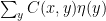, where is translationaly invariant:

Hence is diagonal in the sense previously explained. It is easily calclated to be

Notice that a daggered variable (i.e., a conjugate transpose) appears in the action. We need to take care of this. Since is, in principle, a “real” Grassmann variable, its Fourier transform satisfies . This “Hermitian” property of the Fourier transform of real functions allows us to write the action as

We can explicitly evaluate the needed Berezin integral. But some care is necessary. Observe that the action “mixes” frequencies and . When we rewrite the exponential of the sum in the above action as a product of exponentials of the summands, these exponentials will contain not only the 4 grassman variables that make up the vector , but also the other 4 variables in . So the full Berezin integral will factor not into Berezin integrals over 4 variables, but over 8 variables. So we will regroup the Grassmann differentials in groups of 8 rather than in groups of four, as follows:

In order to correctly factor the full Berezin integral, we need to collect all terms with and , which we can do by rewriting the sum in the action half the values of . We will abuse the notation and write to mean that and are not both included in the summation. For instance, we can accomplish this by taking . With this notation, we can write,

If we define

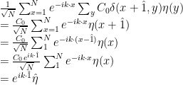
then we can write the action as

Let us write

The full Berezin integral now factors and can be written

Each of the Berezin integral factors is a Gaussian integral. Recall that

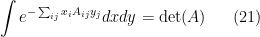
for Grassmann numbers and and a complex matrix (see here for an explanation). So

Removing the restriction to we have

Taking logarithms and dividing by the number of sites we have

In the thermodynamic limit, the sum becomes an integral and the partition function per site

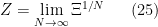
is thus given by

The anti-hermitian matrix is easily found:

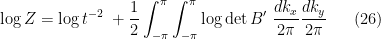
Its determinant is

Substituting into the integral, we arrive at the expression for the partition function per site:

We are done! This is Onsager’s famous result, specialized to the case of of equal coupĺings .

Exercise: Repeat the calculation using the high temperature variable instead of the low tempoerature variable . (The final answer is of course the same.)

5. The cubic Ising model

Ever since 1944 when Onsager published his seminal paper, tentative “exact solutions” have been proposed over the years for the 3D or cubic Ising model. As mentioned eariler, the Grassmann action is quartic for the cubic Ising model. In quantum field theory, quartic Grassmann actions are associated with models of interacting fermions, whereas quadratic actions are associated with free-fermion models. The latter are easily solved via Pfaffian and determinant formulas, as we have done above, but at the present time there are no methods known to be able to give exact solutions (in the thermodynamic limit) of lattice models with quartic Grassmann actions. Hence, anybody claiming an exact solution to the cubic Ising model must explain how they overcame the mathematical difficulty of dealing with quartic actions, or at least how the new method bypasses this mathematical obstruction.

Barry Cipra, in an article in Science, referred to the Ising problem as the “Holy Grail of statistical mechanics.” The article lists a number of other reasons why we may never attain the goal of finding an explicit exact solution of the cubic Ising model.

Exact solution of the cubic Ising model may be an impossible problem!

---

I thank Francisco “Xico” Alexandre da Costa and Sílvio Salinas for calling my attention to the Grassmann variables approach to solving the Ising model.

Fermionization of the 2-D Ising model: The method of Schultz, Mattis and Lieb

F. A da Costa, R. T. G. de Oliveira, G. M. Viswanathan

This blog post was written in co-authorship with my physics department colleague Professor Francisco “Xico” Alexandre da Costa and Professor Roberto Teodoro Gurgel de Oliveira, of the UFRN mathematics department. Xico obtained his doctorate under Professor Sílvio Salinas at the University of São Paulo. Roberto was a student of Xico many years ago, but left physics to study mathematics at IMPA in Rio de Janeiro in 2010. During 2006–2007, Roberto and Xico had written up a short text in Portuguese that included the exact solution of the Ising model on the infinite square lattice using the method of fermion operators developed by Schultz, Mattis and Lieb. With the aim of learning this method, I adapted their text and expanded many of the calculations for my own convenience. I decided to post it on this blog since others might also find it interesting. I have previously written an introduction to the 2-D Ising model here, where I review a combinatorial method of solution.

1. Introduction

The spins in the Ising model can only take on two values, . This behavior is not unlike how the occupation number for some single particle state for fermions can only take on two values, . It thus makes sense to try to solve the Ising model via fermionization. This is what Schultz, Mattis and Lieb accomplished in their well-known paper of 1964. In turn, their method of solution is a simplified version of Bruria Kaufman’s spinor analysis method, which is in turn a simplification of Onsager’s original method.

We will proceed as follows. First we will set up the transfer matrix. Next we will reformulate it in terms of Pauli’s spin matrices for spin- particles. Recall that in quantum field theory boson creation and annihilation operators satisfy the well-known commutation relations of the quantum harmonic oscillator, whereas fermion operators satisfy analogous anticommutation relations. The spin annihilation and creation operators do not anticommute at distinct sites but instead commute, whereas fermion operators must anticommute at different sites. This problem of mixed commutation and anticommutation relations can be solved using a method known as the Jordan-Wigner transformation. This step completes the fermionic reformulation of the 2-D Ising model. To obtain the partition function in the thermodynamic limit, which is the largest eigenvalue of the transfer matrix, one diagonalizes the fermionized transfer matrix using appropriate canonical transformations.

Onsager’s solution of the 2-D Ising model: The combinatorial method

1. Introduction

In this blog post, I derive, step by step, the exact partition function for the ferromagnetic Ising model on the square lattice. The result is celebrated as “Onsager’s solution” of the 2-D Ising model. It was originally derived by Lars Onsager in 1942 and published in 1944 in Physical Review [1]. That paper revolutionized the study of phase transitions and what we now call critical phenomena [2].

Somewhat ironically, I first heard about the Ising model when I was working in industry. I was 20 and held a summer job at what was then known as British Telecom Research Labs (BTRL), near Ipswich in the UK. This was before I had ever seen a cell phone or heard of the Internet (although I knew about BITNET and JANET). I worked there in the summer of 1990 and again for a month or so around April 1991. My job at BT involved writing C implementations of multilayer perceptrons and Hopfield neural nets. In those days, BT was interested in implementing hardware neural networks and my boss mentioned casually to me that certain kinds of neural nets are basically just special cases of the Ising model. (Indeed, the Hopfield network is closely related to the Ising spin glass.) Thus began my fascination with the Ising model. Later, in 1994 in Boston, I took a course given by Bill Klein at BU on statistical mechanics, where we went through the solution of the 1-D ferromagnetic Ising model. Still, I never had the chance to study properly the 2-D Ising model. As a PhD student, I would almost daily pass by a poster with a background photo of Lars Onsager (with a cigarette in his hand), hung near the office door of my advisor Gene Stanley, so I was regularly reminded of the 2-D Ising model. I kept telling myself that one day I would eventually learn how Onsager managed to do what seemed to me, at the time, an “impossible calculation.” That was 1994 and I am writing this in 2015!

In what follows, I solve the Ising model on the infinite square lattice, but I do not actually follow Onsager’s original argument. There are in fact several different ways of arriving at Onsager’s expression [3–9]. The method I use below is known as the combinatorial method and was developed by van der Waerden, Kac and Ward among others and relies essentially on counting certain kinds of closed graphs (see refs. [3,10–13]). I more or less follow Feynman [3] and I have also relied on the initial portions of ref. [13].

2. The 2-D Ising model

Consider a two dimensional lattice where at each point of the lattice is located a (somewhat idealized) spin- particle. Consider a finite subset of this lattice, of size and let . Let denote the set of pairs of integers such that spins and are nearest neighbors. In the ferromagnetic 2-D Ising model with nearest neighbor interactions, spins and interact if and only if . Each spin can assume only 2 values: .

Consider a system of spins. The Hamiltonian for a spin configuration is given by

The sum over the nearest neighbors should avoid double counting, so that and are not counted separately. Without loss of generality, we will assume for simplicity.

3. The canonical partition function

In the theory of equilibrium statistical mechanics, the canonical partition function contains all the information needed to recover the thermodynamic properties of a system with fixed number of particles, immersed in a heat bath, details of which can be found in any textbook on statistical mechanics [3-6,14].

I prefer to define the partition function as the two-sided Laplace transform of the degeneracy of the energy level . But traditionally, the partition function is defined as a sum or integral over all possible states of the system:

The two ways of thinking are equivalent. The Laplace transform variable is related to the thermodynamic temperature via , where is the Boltzmann constant. What follows is the exact calculation of .